
ATLAS e-News
23 February 2011
Simulation slimdown
20 October 2009
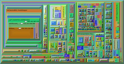
'Callgrind' visual representation of the average CPU demand of five simulated events in ATLAS last year. The nested boxes each
represent different pieces of the code, scaled relative to how much they're used.
The magnetic field code making up the big block on the left was
improved after this Callgrind profile alerted the core simulation
group to its dominance. (Click for full image)
In the run-up to beam, there has been a big effort to optimise both the simulation code and the reconstruction code. This week, we’re looking at the efficiency of the simulation code, where improvements have been made across the board in reducing disk space and memory consumption, as well as CPU demand.
Since all simulated data sent out to the Grid is also stored for potential reprocessing, saving it more efficiently can lead to significant space savings down the line. Compressing the data at the write-out stage – where recording to the standard eight or 16 decimal places is pointless if the detector can only be read to much fewer – has enabled cut backs on essentially wasted disk space, without compromising the accuracy of the data.
“In particular, the TRT changed the way they were doing their storage and got us something like 40 per cent of our disk space free,” reports Zach Marshall, from the core simulation group.
Reining in memory consumption is more of an urgent issue for the reconstruction group at the moment, as reported in the last issue of e-News, but it’s still worth considering for the simulation. Although most Grid machines now have 2GB of memory per core, it’s easier to allocate a queue of 1GB jobs than a queue of 2GB jobs, so effort has been made to shave waste wherever possible. The smaller the memory footprint of an application, the more chance it has of being able to nip into a pocket of available space on a given machine, meaning that more simulations can be run simultaneously.
As with the reconstruction code, a new profiling tool that highlights memory-heavy applications has been instrumental in trimming down memory consumption. Rather than each individual developer wasting time scouring their code for measly savings, the tool picks up on wasteful code that has a big impact through repetition; the inefficiencies may only be tiny, but the code is called on so frequently that it squanders a significant amount of memory over time. Once the areas with greatest potential for improvement have been highlighted, it’s simply a case of tipping off the relevant developers.
Another new diagnostic tool has helped out on the CPU side, looking at how time is spent on jobs. “We found a handful of places where people have written perfectly good code, if the code gets called ten times,” explains Zach. “But in fact it ends up getting called 100 million times, and suddenly things get bad.”
The solution, according to Zach is “to do the coding equivalent of the Google homepage” with these in-demand areas: make the basic parts used by everybody as plain and uncluttered as possible, with the more complex parts used by individual groups hidden away outside of the main code base. Other ‘tricks’ like reordering elements, reducing the number of log messages and making tweaks to some of the detector conditions assumptions have all helped save on CPU time.
“We’ve been doing a little nipping and tucking here and there,” says Zach, “and it turns out, when you do that with something that’s used a lot, you can actually make a big impact on the whole thing.”
A good example of a small tweak making a huge difference is in the case of ‘stuck tracks’. These occur when the Geant4 simulation stalls as it tries to send a particle from one detector volume to another, for example from air into a solid. It occasionally gets thrown by the changes in physical properties between the volumes, and ends up with the particle perpetually going back and forth between them, until the whole job times out after two days and all the output is lost.
This problem was supposedly solved long ago when various triggers were built into the code to un-stick the track after a given number of failed steps. But it seems that, in some cases, simulated particles were shuffling along at fractions of a micrometre at a time and failing to trigger any of that extra logic. A recent altering of the tolerance levels in Geant4, so that it now recognises these cases as essentially ‘stuck’ should hopefully put an end to the problem.
Finally, as well as looking inwards at their code, the core simulation team have also been looking outwards – at our direct competitor, CMS. In a move that was at once sporting and competitive, the experiments decided to run a fair comparison of their simulations, taking the same input, on the same computer, run through the two different simulations.
“We both have a long way to go in making our simulations as fast as they can possibly be,” Zach concedes, but ATLAS came out markedly slower than CMS. Things aren’t black and white though; one of the biggest influencing factors was that ATLAS chose to use a slower physics model for the simulation because, after extensive testing, the ATLAS team agreed that it was the more reliable option.
“We said to ourselves, ‘OK, we’re going to bite the bullet, go with the slower physics list, and try and get things right first go.’ Hopefully that sets us up well for data,” smiles Zach. “Hopefully…”

Ceri PerkinsATLAS e-News
|